
Blog
Turbocharge Your Data Science Workbench


Use Web Components with Jupyter Notebooks
If you are a Data Scientist, you ought to have worked on a Jupyter Notebook. Notebooks are the simplest form of interface to Python, especially if you want to do some Data Science analytics. Notebooks have clearly become one of the most popular tools for Data Scientists. With continuous improvements, more features and enhanced abilities to ingest data from variety of data sources, this tool is here to stay. At the same time, interactivity of web applications, using impressive JavaScript visualization libraries, is reaching newer heights by the day. Inspired by some of the recent developments in the area of Web Components, we came up with an idea to combine these two technologies, and enable Data Scientists to work more efficiently with Jupyter Notebooks, thus getting the best of both tools. So, let’s dive deep in.
 Figure 1 : Blank Notebook.
This is where you start. A blank Jupyter Notebook, ready for action. It is assumed that all necessary software has been installed, including additional package like Pandas, Numpy, Matplotlib etc. Introduction to Data For the purpose of demonstration, we will analyse flight delays from public sources of information. United States Department of Transport (www.bts.gov) has made available Airline On-Time Statistics on its web site. Typically, this data is available within a month. We will analyse the flight delays for the month of July 2017 and will target to build something like the figure below.
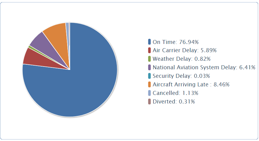 Figure 2 : On-time analysis. Source (www.bts.gov)
There are good analysis and graphic representations on the site. However, as Data Scientists, we always have the curiosity to do further analysis on top of data, using our own algorithms and approaches. The starting point, however, is to match the results first. The raw data is in the form of one line per airline per airport. The file contains 21 fields but for now, we will focus on two which are most relevant i.e. number of flights which landed and, number of flights which were delayed. 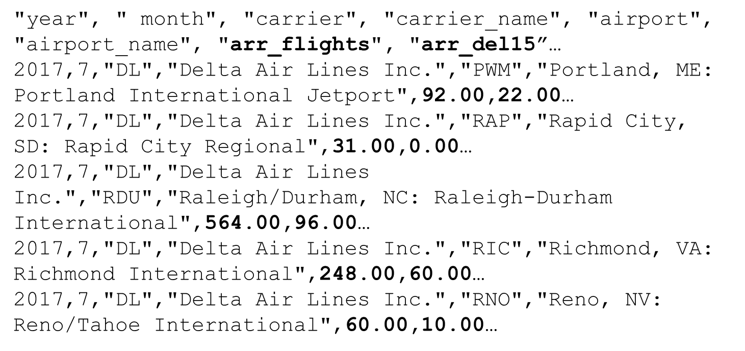 Figure 3 : Snapshot of raw data Prepare for Analysis. Ingest Data in memory Python Pandas is the most obvious choice to read the data and make it ready in memory. Since we already have the data in Comma Separated Values (CSV) format, Pandas has a ready made support for it.
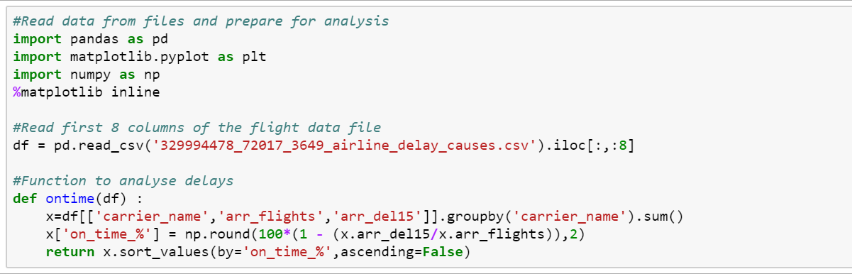 Figure 4 : Python code to read the data about Flights Delay
The code is rather simple. All it needs, is one line of code to read and prepare the CSV file in memory. We will come to the use of “ontime” function, little later. As soon as this cell is executed, a Dataframe representation is available as a variable named “df”. Build the re-usable Web Component There are two parts to it. And that’s the whole idea of bringing two technologies together. First, write up the component in JavaScript using Web Components standard. This is a small extract of the code.
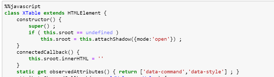 Figure 5 : Create a Class in JavaScript
Jupyter Notebook allows the use of JavaScript code in its cells, using %%javascript. In this example, we have defined a class. The class can also define a ‘constructor’ and we have used the concept of “Shadow Root” in the constructor. This web component can be triggered whenever its properties “data-command” and “data-style” are changed. While we have used the Notebook cell to code the component, it is also possible to create the entire code in an external JS file and reuse it in multiple notebooks. Next, in the JavaScript code, use the full power of Notebook kernel using the, relatively less documented, IPython.notebook.kernel engine. Its ‘execute’ function has some specific nuances, which if followed, work well.
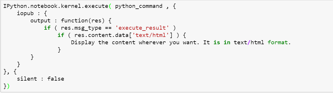 Figure 6 : Use IPython’s kernel to fetch data from underlying Python engine
First parameter of the execute call, can be a simple Python command, e.g. df.head() or, a function e.g. ontime(df) as above. That’s it. This needs to be done only once. Now we are ready to use the component. Please note that the code pieces above, just illustrate the concepts. The entire working code, can be downloaded from here. Use the component in Jupyter Notebooks And it all boils down to one line of code
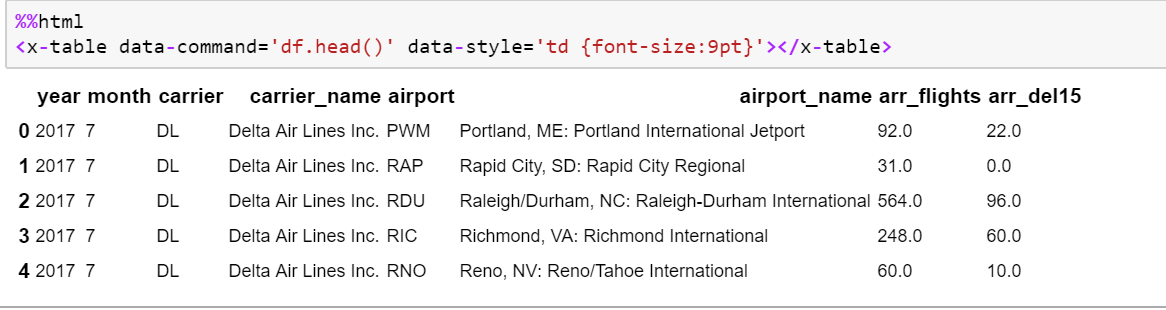 Figure 7 : Using the custom x-table tag
From here on, you can combine your HTML creativity to build a highly interactive application, which looks and behaves like a web application but still, combines the high power of Python and Jupyter Notebook to deliver a Data Science application. We were able to build an interactive web application under Jupyter such that a use can select the various options from a dropdown menu and can see the results immediately, without clicking on the any of IPython hot buttons like “Run”. Like other web applications which react to change in a text input, we could connect the text entered, with the query, and deliver the results instantly. Here are some snapshots from the final Notebook.
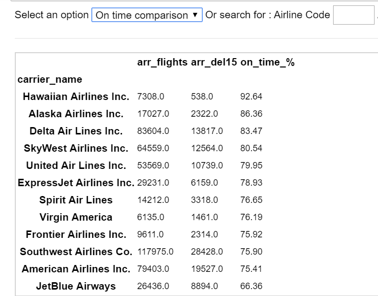 Figure 8 : Custom component can display summary of Dataframe
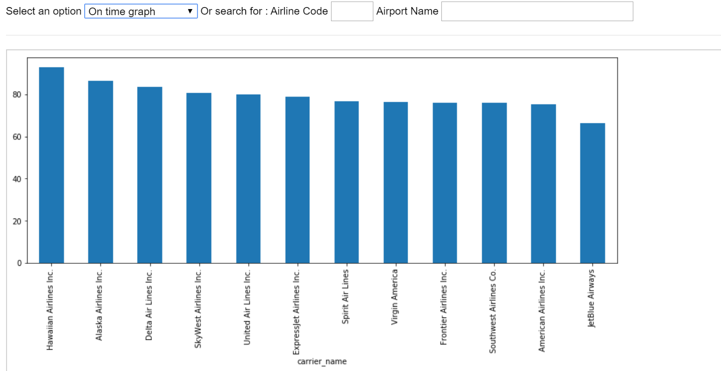 Figure 9 : Custom component can also display a graph
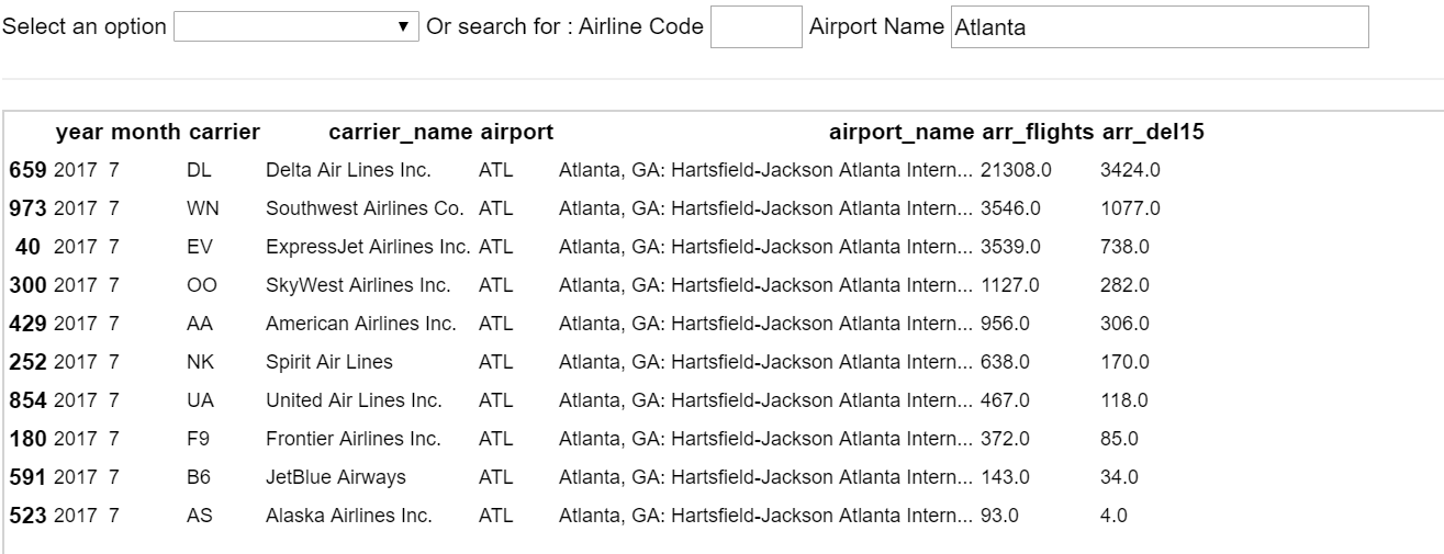 Figure 10 : Custom component can also react to changes in HTML input fields.
In conclusion This blog, is one more in the series of blogs related to Web Components. Even though the standards are being finalized and implemented, the combination of Web Components with Jupyter Notebooks has tremendous potential in today’s Data Science development work. References
- Custom Elements v1: Reusable Web Components by Eric Bidelman (Developers.google.com)
- Airline On-Time Statistics (Transtats.bts)
- Install Python 3 (Python.org), Jupyter(Jupyter.org), Pandas (Pandas.pydata) and Matplotlib (Matplotlib).


Get Started


