
Blog
Decision Trees for Classification: A Machine Learning Algorithm
Blog
Decision Trees for Classification: A Machine Learning Algorithm


Introduction Decision Trees are a type of Supervised Machine Learning (that is you explain what the input is and what the corresponding output is in the training data) where the data is continuously split according to a certain parameter. The tree can be explained by two entities, namely decision nodes and leaves. The leaves are the decisions or the final outcomes. And the decision nodes are where the data is split. While a single Decision Tree is easy to interpret, ensemble techniques like the Random Forest algorithm often deliver more stable and accurate predictions in real-world scenarios.
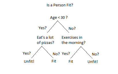
An example of a decision tree can be explained using above binary tree. Let’s say you want to predict whether a person is fit given their information like age, eating habit, and physical activity, etc. The decision nodes here are questions like ‘What’s the age?’, ‘Does he exercise?’, ‘Does he eat a lot of pizzas’? And the leaves, which are outcomes like either ‘fit’, or ‘unfit’. In this case this was a binary classification problem (a yes no type problem). There are two main types of Decision Trees:
- Classification trees (Yes/No types)
What we’ve seen above is an example of classification tree, where the outcome was a variable like ‘fit’ or ‘unfit’. Here the decision variable is Categorical.
- Regression trees (Continuous data types)
Here the decision or the outcome variable is Continuous, e.g. a number like 123. Working Now that we know what a Decision Tree is, we’ll see how it works internally. There are many algorithms out there which construct Decision Trees, but one of the best is called as ID3 Algorithm. ID3 Stands for Iterative Dichotomiser 3. Before discussing the ID3 algorithm, we’ll go through few definitions.
- Entropy:
Entropy, also called as Shannon Entropy is denoted by H(S) for a finite set S, is the measure of the amount of uncertainty or randomness in data. 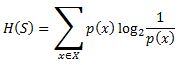 Intuitively, it tells us about the predictability of a certain event. Example, consider a coin toss whose probability of heads is 0.5 and probability of tails is 0.5. Here the entropy is the highest possible, since there’s no way of determining what the outcome might be. Alternatively, consider a coin which has heads on both the sides, the entropy of such an event can be predicted perfectly since we know beforehand that it’ll always be heads. In other words, this event has no randomness hence it’s entropy is zero. In particular, lower values imply less uncertainty while higher values imply high uncertainty.
- Information Gain:
nformation gain is also called as Kullback-Leibler divergence denoted by IG(S,A) for a set S is the effective change in entropy after deciding on a particular attribute A. It measures the relative change in entropy with respect to the independent variables. ![]() Alternatively,
Alternatively, 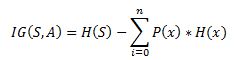 where IG(S, A) is the information gain by applying feature A. H(S) is the Entropy of the entire set, while the second term calculates the Entropy after applying the feature A, where P(x) is the probability of event x.
Let’s understand this with the help of an example. Consider a piece of data collected over the course of 14 days where the features are Outlook, Temperature, Humidity, Wind and the outcome variable is whether Golf was played on the day. Now, our job is to build a predictive model which takes in above 4 parameters and predicts whether Golf will be played on the day. We’ll build a decision tree to do that using ID3 algorithm.
In production, decision tree models almost never train on a 14-day sample like this - real-world models pull from datasets of millions of observations, often collected through web scraping infrastructure that aggregates public data across thousands of sources before any feature engineering begins.
| Day | Outlook | Temperature | Humidity | Wind | Play Golf |
| D1 | Sunny | Hot | High | Weak | No |
| D2 | Sunny | Hot | High | Strong | No |
| D3 | Overcast | Hot | High | Weak | Yes |
| D4 | Rain | Mild | High | Weak | Yes |
| D5 | Rain | Cool | Normal | Weak | Yes |
| D6 | Rain | Cool | Normal | Strong | No |
| D7 | Overcast | Cool | Normal | Strong | Yes |
| D8 | Sunny | Mild | High | Weak | No |
| D9 | Sunny | Cool | Normal | Weak | Yes |
| D10 | Rain | Mild | Normal | Weak | Yes |
| D11 | Sunny | Mild | Normal | Strong | Yes |
| D12 | Overcast | Mild | High | Strong | Yes |
| D13 | Overcast | Hot | Normal | Weak | Yes |
| D14 | Rain | Mild | High | Strong | No |
ID3 Algorithm will perform following tasks recursively
- Create root node for the tree
- If all examples are positive, return leaf node ‘positive’
- Else if all examples are negative, return leaf node ‘negative’
- Calculate the entropy of current state H(S)
- For each attribute, calculate the entropy with respect to the attribute ‘x’ denoted by H(S, x)
- Select the attribute which has maximum value of IG(S, x)
- Remove the attribute that offers highest IG from the set of attributes
- Repeat until we run out of all attributes, or the decision tree has all leaf nodes.
Now, let's go ahead and grow the decision tree. The initial step is to calculate H(S), the Entropy of the current state. In the above example, we can see in total there are 5 No’s and 9 Yes’s.
| Yes | No | Total |
| 9 | 5 | 14 |
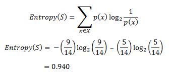
Remember that the Entropy is 0 if all members belong to the same class, and 1 when half of them belong to one class and other half belong to other class that is perfect randomness. Here it’s 0.94 which means the distribution is fairly random. Now, the next step is to choose the attribute that gives us highest possible Information Gain which we’ll choose as the root node. Let’s start with ‘Wind’ 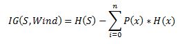
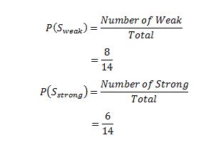
where ‘x’ are the possible values for an attribute. Here, attribute ‘Wind’ takes two possible values in the sample data, hence x = {Weak, Strong} We’ll have to calculate:  Amongst all the 14 examples we have 8 places where the wind is weak and 6 where the wind is Strong.
| Wind = Weak | Wind = Strong | Total |
| 8 | 6 | 14 |
Now, out of the 8 Weak examples, 6 of them were ‘Yes’ for Play Golf and 2 of them were ‘No’ for ‘Play Golf’. So, we have, 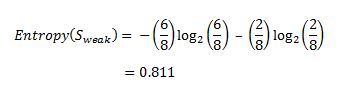 Similarly, out of 6 Strong examples, we have 3 examples where the outcome was ‘Yes’ for Play Golf and 3 where we had ‘No’ for Play Golf.
 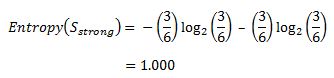 Remember, here half items belong to one class while other half belong to other. Hence we have perfect randomness. Now we have all the pieces required to calculate the Information Gain,
 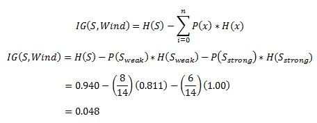 Which tells us the Information Gain by considering ‘Wind’ as the feature and give us information gain of 0.048. Now we must similarly calculate the Information Gain for all the features.
 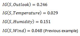 We can clearly see that IG(S, Outlook) has the highest information gain of 0.246, hence we chose Outlook attribute as the root node. At this point, the decision tree looks like.
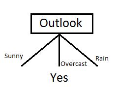
Here we observe that whenever the outlook is Overcast, Play Golf is always ‘Yes’, it’s no coincidence by any chance, the simple tree resulted because of the highest information gain is given by the attribute Outlook. Now how do we proceed from this point? We can simply apply recursion, you might want to look at the algorithm steps described earlier. Now that we’ve used Outlook, we’ve got three of them remaining Humidity, Temperature, and Wind. And, we had three possible values of Outlook: Sunny, Overcast, Rain. Where the Overcast node already ended up having leaf node ‘Yes’, so we’re left with two subtrees to compute: Sunny and Rain. ![]() Table where the value of Outlook is Sunny looks like:
Table where the value of Outlook is Sunny looks like:
| Temperature | Humidity | Wind | Play Golf |
| Hot | High | Weak | No |
| Hot | High | Strong | No |
| Mild | High | Weak | No |
| Cool | Normal | Weak | Yes |
| Mild | Normal | Strong | Yes |
![]() In the similar fashion, we compute the following values
In the similar fashion, we compute the following values 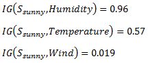 As we can see the highest Information Gain is given by Humidity. Proceeding in the same way with
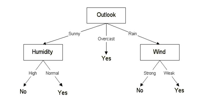
 ![]() will give us Wind as the one with highest information gain. The final Decision Tree looks something like this.
will give us Wind as the one with highest information gain. The final Decision Tree looks something like this.
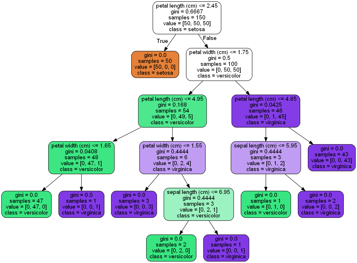
Code: Let’s see an example in Python
import pydotplus
 from sklearn.datasets import load_iris
 from sklearn import tree
 from IPython.display import Image, display
__author__ = "Mayur Kulkarni <mayur.kulkarni@xoriant.com>"

 def load_data_set():
    """
    Loads the iris data set

    :return:        data set instance
    """
   iris = load_iris()
    return iris

 def train_model(iris):
    """
    Train decision tree classifier

    :param iris:    iris data set instance
    :return:        classifier instance
    """
   clf = tree.DecisionTreeClassifier()
    clf = clf.fit(iris.data, iris.target)
    return clf

 def display_image(clf, iris):
    """
    Displays the decision tree image

    :param clf:     classifier instance
    :param iris:    iris data set instance
    """
   dot_data = tree.export_graphviz(clf, out_file=None,
                                    feature_names=iris.feature_names,
                                    class_names=iris.target_names,
                                    filled=True, rounded=True)

    graph = pydotplus.graph_from_dot_data(dot_data)
    display(Image(data=graph.create_png()))

 if __name__ == '__main__':
    iris_data = load_iris()
    decision_tree_classifier = train_model(iris_data)
    display_image(clf=decision_tree_classifier, iris=iris_data)
 Conclusion: Below is the summary of what we’ve studied in this blog:
- Entropy to measure discriminatory power of an attribute for classification task. It defines the amount of randomness in attribute for classification task. Entropy is minimal means the attribute appears close to one class and has a good discriminatory power for classification
- Information Gain to rank attribute for filtering at given node in the tree. The ranking is based on high information gain entropy in decreasing order.
- The recursive ID3 algorithm that creates a decision tree.
References:
- Information Gain: Wikipedia.org
- Entropy: Wikipedia.org
- ID3: Wikipedia.org
- Entropy YouTube video: Youtube.com
- ID3 Example: Cise.ufl.edu
To explore how Decision Trees and similar models fit into the broader journey of enterprise AI, read Artificial Intelligence Tree: Mapping Enterprise AI Evolution
.
This article illustrates how AI adoption in enterprises evolves like a growing tree — where data and governance form the roots, AI and ML models (like Decision Trees) make up the trunk, and real business applications represent the fruit. It emphasizes that a strong foundation in data quality, scalable architecture, and operationalized AI (MLOps, DataOps) is essential before advanced AI initiatives can deliver measurable business value.
If you're looking for a more robust approach that reduces overfitting and improves predictive stability, explore our detailed guide on the Random Forest algorithm in machine learning.


Get Started


